ANSWERS TO HOMEWORK QUESTIONS

Chapter 3
Review Questions
1.   A production function shows how much output can be produced with a given amount of capital and labor. The production function can shift due to supply shocks, which affect overall productivity. Examples include changes in energy supplies, technological breakthroughs, and management practices. Besides knowing the production function, you must also know the quantities of capital and labor the economy has.
2.   The upward slope of the production function means that any additional inputs of capital or labor produce more output. The fact that the slope declines as we move from left to right illustrates the idea of diminishing marginal productivity. For a fixed amount of capital, additional workers each add less additional output as the number of workers increases. For a fixed number of workers, additional capital adds less additional output as the amount of capital increases.
3.   The marginal product of capital (MPK) is the output produced per unit of additional capital. The MPK can be shown graphically using the production function. For a fixed level of labor, plot the output provided by different levels of capital; this is the production function. The MPK is just the slope of the production function.
4.   The marginal revenue product of labor represents the benefit to a firm of hiring an additional worker, while the nominal wage is the cost. Comparing the benefit to the cost, the firm will hire additional workers as long as the marginal revenue product of labor exceeds the nominal wage, since doing so increases profits. Profits will be at their highest when the marginal revenue product of labor just equals the nominal wage.
The same condition can be expressed in real terms by dividing through by the price of the good. The resulting equation shows that the real wage (W/P) equals the marginal product of labor.
12. Frictional unemployment arises as workers and firms search to find matches. A certain amount of frictional unemployment is necessary, because it is not always possible to find the right match right away. For example, an unemployed banker may not want to take a job flipping hamburgers if she cannot find another banking job right away, because the match would be very poor. By remaining unemployed and continuing to search for a more suitable job, the banker is likely to make a better match. That will be better both for the banker (because the salary is likely to be higher) and for society as a whole (because the better match means greater productivity in the economy).
13. Structural unemployment occurs when people suffer long spells of unemployment or are chronically unemployed. Structural unemployment arises when the number of potential workers with low skill levels exceeds the number of jobs requiring low skill levels, or when the economy undergoes structural change.  When there is structural change, workers who lose their jobs in shrinking industries may have to move to find new jobs.
14. The natural rate of unemployment is the rate of unemployment that prevails when output and employment are at their full-employment levels. The natural rate of unemployment is equal to the amount of frictional unemployment plus structural unemployment. Cyclical unemployment is the difference between the actual rate of unemployment and the natural rate of unemployment. When cyclical unemployment is negative, output and employment exceed their full-employment levels.
15. Okun’s Law is a rule of thumb that tells how much output falls when the unemployment rate rises.  Specifically, it says that the percentage change in GDP equals 3 minus 2 times the change in the unemployment rate.  If the unemployment rate increases by two percentage points, the percentage change in GDP will be 3 – 2(2) = -1.

 

 

 

 

 

 

Numerical problems
3.   (a)

N	Y	MPN	MRPN (P = 5)	MRPN (P = 10)
1	8	8	40	80
2	15	7	35	70
3	21	6	30	60
4	26	5	25	50
5	30	4	20	40
6	33	3	15	30

      (b) P = $5.
(1) W = $38. Hire one worker, since MRPN ($40) is greater than W ($38) at N = 1. Do not hire two workers, since MRPN ($35) is less than W ($38) at N = 2.
(2) W = $27. Hire three workers, since MRPN ($30) is greater than W ($27) at N = 3. Do not hire four workers, since MRPN ($25) is less than W ($27) at N = 4.
(3)  W = $22. Hire four workers, since MRPN ($25) is greater than   W ($22) at N = 4. Do not hire five workers, since MRPN ($20) is less than W ($22) at N = 5.

(c) Figure 1 plots the relationship between labor demand and the nominal wage. This graph is different from a labor demand curve because a labor demand curve shows the relationship between labor demand and the real wage. Figure 2 shows the labor demand curve.

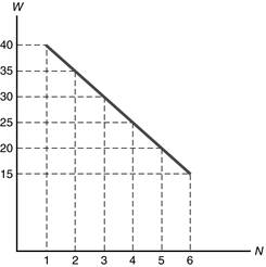
Figure 1
 
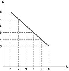
Figure 2

(d) P = $10. The table in part (a) shows the MRPN for each N. At W = $38, the firm should hire five workers. MRPN ($40) is greater than W ($38) at N = 5. The firm shouldn’t hire six workers, since MRPN ($30) is less than W ($38) at N = 6. With five workers, output is 30 widgets, compared to 8 widgets in part (a) when the firm hired only one worker. So the increase in the price of the product increases the firm’s labor demand and output.

(e) If output doubles, MPN doubles, so MRPN doubles. The MRPN is the same as it was in part (d) when the price doubled. So labor demand is the same as it was in part (d). The output produced by five workers now doubles to 60 widgets.

(f)  Since MRPN = P ´ MPN, then a doubling of either P or MPN leads to a doubling of MRPN. Since labor demand is chosen by setting MRPN equal to W, the choice is the same, whether P doubles or MPN doubles.

Analytical problems

2.  (a) An increase in the number of immigrants increases the labor force, increasing employment and increasing full-employment output.
(b) If energy supplies become depleted, it is likely to reduce productivity, because energy is a factor of production. So the reduction in energy supplies reduces full-employment output.
(c) Better education raises future productivity and output, but has no effect on current full-employment output.
(d) The reduction in the capital stock reduces full-employment output (although it may very well increase overall welfare).

Chapter 4
Review Questions
1.   Saving is current income minus consumption. For a given income, any increase in consumption means an equal decrease in saving, so consumption and saving are inversely related. The basic motivation for saving is to provide for future consumption.

2.  When a consumer gets an increase in current income, both current consumption and future consumption increase. That means part of the additional current income will be spent and part will be saved. When the consumer gets an increase in expected future income, again both current and future consumption increase. Because current income does not increase, but current consumption does, saving decreases. When the consumer gets an increase in wealth, both current and future consumption again rise. Again, there has been no increase in current income, so saving decreases.
3.  An increase in the real interest rate has two effects on desired saving: (1) The substitution effect increases saving, because the amount of future consumption that can be obtained in exchange for giving up a unit of current consumption rises.  (2) The income effect may increase or reduce saving. The income effect reduces saving for a lender, because a person who saves is better off as a result of having a higher real interest rate, so he or she increases current consumption. However, for a borrower, the income effect increases saving, because the borrower is worse off with a higher real interest rate. So the income effect works in different directions depending on whether a person is a lender or a borrower. For a borrower, then, both the income and substitution effects work in the same direction, and saving definitely increases. For a lender, the income and substitution effects work in opposite directions, so the result on desired saving is ambiguous.

4.  The expected after-tax real interest rate equals (1 – t)i – Πe , where t is the tax rate, i is the nominal interest rate, and Πe is the expected inflation rate.  If the tax rate declines, then the expected after-tax real interest rate will rise.

6.  The two components of the user cost of capital are the interest cost and the depreciation cost. The depreciation cost is the value lost as the capital wears out during the period. The interest cost represents the opportunity cost of using the funds to purchase capital instead of another asset, such as a bond

7.  The desired capital stock is the amount of capital that allows the firm to earn the largest possible profit. The higher the expected future marginal product of capital, the higher the desired capital stock, because any given amount of capital will be more productive in the future. The higher the user cost of capital, the lower the desired capital stock, because a higher user cost yields lower profits on each unit of capital. The higher the effective tax rate, the lower the desired capital stock, because the firm gets lower profits on each unit of capital.

8.  Gross investment is the total purchase of new capital goods during a specified period. Net investment is gross investment minus the depreciation on existing capital. Net investment is the overall increase in the capital stock. Yes, it is possible for gross investment to be positive when net investment is negative. This occurs whenever gross investment is less than the amount of depreciation (as happened in the United States during World War II).
9.   Equilibrium in the goods market occurs when the aggregate supply of goods (Y) equals the aggregate demand for goods (Cd + Id + G). Since desired national saving (Sd) is Y – Cd – G, an equivalent condition is Sd = Id. Equilibrium is achieved by the adjustment of the real interest rate to make the desired level of saving equal to the desired level of investment.  The relevant diagram is:

Numerical Problems
5.  (a) Desired consumption declines as the real interest rate rises because the higher return to saving encourages higher saving; desired investment declines as the real interest rate rises becauses the user cost of capital is higher, reducing the desired capital stock, and thus investment.
(b) Recall that Sd = Y – Cd – G, so Sd = 9000 – Cd – 2000 = 7000 – Cd .

r	Cd	Id	Sd	Cd +Id +G
2	6100	1500	900	9600
3	6000	1400	1000	9400
4	5900	1300	1100	9200
5	5800	1200	1200	9000
6	5700	1100	1300	8800

     (c) Y = Cd + Id + G at equilibrium. Given Y = 9,000, the equilibrium condition holds only at r = 5%. At r = 5% it is also true that Sd = Id = 1200.

     (d) When government purchases fall by 400 to 1600, each Sd entry in the table is higher by 400, and each Cd + Id + G entry is lower by 400. Then Y = Cd + Id + G occurs at r = 3%, and Sd = Id = 1400 at r = 3%.

r	Cd	Id	Sd	Cd +Id +G
2	6100	1500	1300	9200
3	6000	1400	1400	9000
4	5900	1300	1500	8800
5	5800	1200	1600	8600
6	5700	1100	1700	8400

 

Analytical Problems

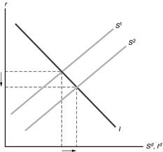
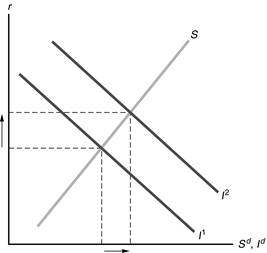
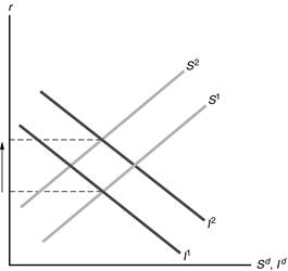
1.   (a) The saving curve shifts to the right from S1 to S2.  Saving and investment increase and the real interest rate falls.

     (b) This is really just a transfer from the general population to veterans. The effect on saving depends on whether the marginal propensity to consume (MPC) of veterans differs from that of the general population. If there is no difference in MPCs, then there will be no shift of the saving curve; neither investment nor the real interest rate is affected. If the MPC of veterans is higher than the MPC of the general population, then desired national saving declines and the saving curve shifts to the left; the real interest rate rises and investment declines. If the MPC of veterans is lower than that of the general population, the saving curve shifts to the right; the real interest rate declines and investment rises.
(c)  The investment tax credit encourages investment, shifting the investment curve from I1 to I2. Saving and investment increase, as does the real interest rate.

 

(d)   The increase in expected future income decreases current desired saving, as people increase desired consumption immediately. The rise of the future marginal productivity of capital shifts the investment curve to the right. As a result, the real interest rate rises, with ambiguous effects on saving and investment.

 

 

 

Chapter 5

Review Questions
1.   Credit items in the current account are exports of goods and services, income receipts from abroad and incoming unilateral transfers.  Debit items in the current account are imports of goods and services, income payments to foreigners, and outgoing unilateral transfers. Adding all of the credit items and subtracting all of the debit items gives the current account balance. The current account balance equals net exports plus net income from abroad plus net unilateral transfers.
2.   The current account includes only the trade of currently produced goods, services and resources, plus unilateral transfers. Trades of existing assets are counted in the capital and financial account.

5.   In a small open economy, saving does not have to be equal to investment. Saving can be used to finance domestic investment or it can be lent abroad. So saving equals investment plus net exports.
Similarly, output need not equal absorption. Absorption is a country’s total spending on consumption, investment, and government purchases. Absorption may be different from output because some output may be exported. The difference between output and absorption is net exports.
8.   An increase in desired national saving in a large open economy reduces the world real interest rate. The saving curve shifts to the right which increases the country’s current account at the current world real interest rate. To restore equilibrium, the world real interest rate must fall.
An increase in desired investment has the opposite effect. The increase in investment reduces the domestic country’s current account and leads to an increase in the world real interest rate to restore equilibrium.
Saving and investment in small open economies are so small relative to saving and investment in the world that changes in them have very little impact on world markets. On the other hand, a large open economy may account for a substantial fraction of the world’s saving and investment, so a change there has a significant impact.
10. The twin deficits are the government budget deficit and the current account deficit. They are connected because an increase in the government budget deficit reduces national saving, which leads to an increased current account deficit. So the government budget deficit and the current account deficit move in the same direction.

Numerical Problems
1.   

Current Account	Credit	Debit
Goods	100	125
Services	90	80
Income receipts and payments	110	150
Total	300	355

Net exports (NX) = (100 + 90) – (125 + 80) = –15.
Current account balance (CA) = 300 – 355 = –55.

Current and Financial Account	Credit	Debit
Increase in home country assets abroad		160
Increase in foreign assets in home country	200
Total	200	160

Note that the increase in home reserve assets is just a subcategory of the increase in home country assets, so it is not included separately. Similarly, the increase in foreign reserve assets is just a subcategory of the increase in foreign assets in the home country. The information about the changes in home and foreign reserve assets is included for calculation of the official settlements balance only.  It does not affect the capital and financial account.
Capital and financial account balance (KFA) = 200 – 160 = 40.

Statistical discrepancy (SD):
CA + KFA + SD = 0
–55 + 40 + SD = 0
SD = 15

Official settlements balance = 30 – 35 = -5

 

 

Analytical Problems
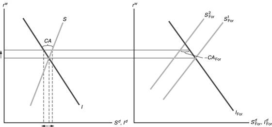
5.     (a) The home country’s saving curve shifts to the right, from S1 to S2. The real world interest rate falls, so that the current account surplus in the home country equals the current account deficit in the foreign country. National S rises, I rises, CA rises, rw falls.


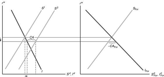
(b) The foreign country’s saving curve shifts to the right, from S1For to S2For. The real world interest rate must fall, so the current account surplus in the foreign country equals the current account deficit in the home country. National S falls, I rises, CA falls, rw falls.

 

 

 

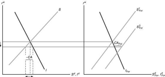
        (c) The foreign country’s saving curve shifts to the left, from S1For to S2For. The real world interest rate must rise, so the current account deficit in the foreign country equals the current account surplus in the home country. National S rises, I falls, CA rises, rw rises.

(d)  If Ricardian equivalence holds, there is no effect. If Ricardian equivalence does not hold, then the result is the same as in part (b), as the foreign country’s saving curve shifts to the right.  That is because all else equal, higher taxes increase government saving more than they reduce private saving.

Chapter 6
Review Questions
1.   The three sources of economic growth are capital growth, labor growth, and productivity growth. The growth accounting approach is derived from the production function.
5.   If there is no productivity growth, then output per worker, consumption per worker, and capital per worker will all be constant in the long run.
6.   The statement is false. Increases in the capital-labor ratio increase consumption per worker in the steady state only up to a point. If the capital-labor ratio is above its golden rule value, then consumption per worker will decline as the capital-labor ratio rises.

 

7.    (a) As long as the capital-labor ratio is below its golden rule value, an increase in the saving rate increases long-run living standards, as higher saving allows for more investment and a larger capital stock.
(b) An increase in the population growth rate reduces long-run living standards, as more output must be used to equip the larger number of new workers with capital, leaving less output available to increase consumption or capital per worker.
(c) A one-time increase in productivity increases living standards directly, by increasing output, and indirectly, because by raising incomes it also raises saving and the capital stock.

Numerical Problems
1.   Hare: $5000 ´ (1.03)50 = $21,919.50
Tortoise: $5000 ´ (1.01)50 = $8,223.15
2.   

	20 Years Ago	Today	Percent Change
Y	1000	1300	30%
K	2500	3250	30%
N	500	575	15%

        (a) DA/A = DY/Y – aK DK/K – aN DN/N
= 30% – (0.3 ´ 30%) - 0.7 ´ 15%
= 30% – 9% – 10.5%
= 10.5%
Capital growth contributed 9% (aK DK / K), labor growth contributed 10.5% (aN DN / N), productivity growth was 10.5%.
(b) DA/A = 30% – (0.5 ´ 30%) - (0.5 ´ 15%)
= 30% – 15% – 7.5%
= 7.5%
Capital growth contributed 15% (aK DK / K), labor growth contributed 7.5% (aN DN / N), productivity growth was 7.5%.

5.   The condition for the steady state is:
sAf(k) = (n + d)k

(a) .3(3k.5) = (.05 + .1)k

           .9k.5 = .15k

           6k.5 = k   so k = 36

           y = 3k.5 = 3(6) = 18

           c = y – i = y – sy = 18 - .3(18) = 12.6

      (b)  Using the same method as in (a),

            k = 64, y = 24, c = 14.4

      (c)  Using the same method as in (a),

            k = 25, y = 15, c = 10.5

      (d)  Using the same method as in (a),

            k = 64, y = 32, c = 22.4       

6.   In the steady state, sAf(k) = (n + d)k, so

      (a)  .1(6k.5) = (.01 + .14)k
.6k.5 = .15k
4k.5 = k
k = 16
y = 6k.5 = 6(4) = 24
c = y – i = y – sy = 24 - .1(24) = 21.6
i = sy =.1(24) = 2.4

      (b) To double output per worker, y must rise from 24 to 48.
y = 6k.5  so k must satisfy the equation 48 = 6k.5.  That implies that k = 64.  To raise k to 64, s must rise.  The new steady state requires that
s6(64.5) = (.01 + .14)64
s48 = 9.6
s = .2

 

 

 

Analytical problems

1.  (a) The destruction of some of a country’s capital stock in a war would have no effect on the steady state, because there has been no change in s, f, n, or d. Instead, k is reduced temporarily, but equilibrium forces eventually drive k to the same steady-state value as before.  The rapid recovery of Germany and Japan after WWII illustrate the point.

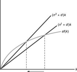
        (b) Immigration raises n from n1 to n2 in the figure below. The rise in n lowers steady-state k, leading to a lower steady-state consumption per worker.

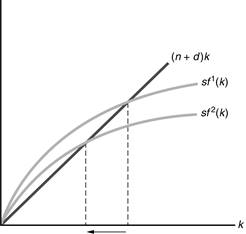
      (c) The rise in energy prices reduces the productivity of capital per worker. This causes sf(k) to shift down from sf1(k) to sf2(k) in the figure below. The result is a decline in steady-state k. Steady-state consumption per worker falls for two reasons: (1) Each unit of capital has a lower productivity, and (2) steady-state k is reduced.

        (d) A temporary rise in s has no effect on the steady-state equilibrium.
(e) The increase in the labor force participation rate does not affect the growth rate of the labor force, so there is no impact on the steady-state capital-labor ratio or on consumption per worker. However, because a larger fraction of the population is working, consumption per person increases.
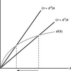
2.   (a) The rise in capital depreciation shifts up the (n + d)k line from (n + d1)k to (n + d2)k, as shown in the figure below. The equilibrium steady-state capital-labor ratio declines. With a lower capital-labor ratio, output per worker is lower, so consumption per worker is lower. There is no effect on the long-run growth rate of the total capital stock, because in the long run the capital stock must grow at the same rate (n) as the labor force grows, so that the capital-labor ratio is constant.

(b)  In an endogenous growth model, the growth rate of output is Dy/y = sA – (n + d), so the rise in the depreciation rate reduces the economy’s growth rate. Similarly, the growth rate of capital equals Dk/k = sA – (n+ d), which also declines when the depreciation rate rises. Since consumption is a constant fraction of output, its growth rate declines as well. So the increase in the depreciation rate reduces the long-run growth rate of the capital stock, as well as long-run capital, output, and consumption per worker.

 

 

Chapter 7
Review Questions
2.   (1) The medium of exchange function allows people to make trades at a lower cost in time and effort than in a barter economy. (2) The unit of account function provides a single, uniform measure of value. (3) The store of value function provides a way of holding wealth that has high liquidity and little risk.
4.   The four characteristics of assets that are most important to wealth holders are (1) expected return, (2) risk, (3) liquidity, and (4) time to maturity. Money has a low expected return compared to other assets.  The level of risk associated with money depends on the probability of unexpected inflation.  Money is the most liquid of all assets, and has zero time to maturity.

6.   The macroeconomic variables that have the greatest impact on money demand are the price level, real income, and the nominal interest rate on other assets. The higher the price level, the higher the demand for money, because more units of money are needed to carry out transactions. The higher the level of real income, the greater the volume of transactions, and so money demand is higher. The higher the nominal interest rate on other assets, the lower is money demand.  That is because the rate of interest is the opportunity cost of holding money.
9.   In equilibrium, the price level is proportional to the nominal money supply.  Specifically, the price level equals the nominal money supply divided by real money demand. The inflation rate is equal to the growth rate of the nominal money supply minus the growth rate of real money demand.

Numerical problems
2.   (a) Real money demand is
Md/P = 500 + 0.2Y – 1000i
= 500 + (0.2 ´ 1000) – (1000 ´ 0.10)
= 600.

         Nominal money demand is
         Md = (Md/P) ´ P = 600 ´ 100 = 60,000.

         In equilibrium, Md = Ms, so velocity is
         V = PY/Md = 100 ´ 1000/60,000 = 1.67.

  (b) Real money demand is unchanged, because neither Y nor i have changed.
Nominal money demand is
       Md = (Md/P) ´ P = 600 ´ 200 = 120,000.
Velocity is unchanged, because neither Y nor Md/P has changed, and we can write the equation for velocity as
           V = PY/Md = Y/(Md/P).
7.   (a) With a constant real interest rate and zero expected inflation, inflation is given by the equation
p = DM/M – hY DY/Y.
To get inflation equal to zero, the central bank should set money growth so that
DM/M = hY DY/Y = 2/3 ´ .045 = .03 = 3%.
The interest elasticity isn’t relevant, since interest rates are expected to remain constant.

Analytical problems

1. (c)  Stocks are an alternative asset to money.  When the expected return to stocks falls, money demand will increase.  People will invest less in stocks and more in cash, checking accounts, and other items that provide liquidity and safety, so the demand for M1 and M2 will rise.

4. For all of these, it is useful to remember that in equilibrium, the price level equals the nominal money supply divided by real money demand.
(a)  An increase in government purchases reduces national saving, causing the real interest rate to rise for a fixed level of income. If the real interest rate is higher, then real money demand will be lower. The price level must rise.  The result is that output is unchanged, the real interest rate increases, and the price level increases.
(b) When expected inflation falls, real money demand increases. There is no effect on employment, saving or investment, so output and the real interest rate remain unchanged. With higher real money demand and an unchanged nominal money supply, the equilibrium price level must decline.

     (c) When labor supply rises, full-employment output increases. Higher output means higher income, so saving will increase.  More saving means the real interest rate will decline. Both higher output and a lower real interest rate increase real money demand.  Higher money demand with a constant money supply means the price level must decline.

• When the interest rate paid on money increases, real money demand rises. That is because the cost of holding money falls.  With no effect on employment or saving and investment, output and the real interest rate remain unchanged. With higher real money demand and an unchanged nominal money supply, the equilibrium price level must decline.

Chapter 9
Review Questions
1.   The labor market and the production function determine the position of the FE line. The equilibrium level of employment is determined in the labor market.  Plugging the equilibrium level of employment into the production function gives the full-employment level of output. The FE line is vertical at that point. The FE line shifts to the right if there is an increase in labor supply, an increase in the capital stock or if there is a beneficial supply shock.

2.  The IS curve shows combinations of the real interest rate (r) and output (Y) where the goods market is in equilibrium. Equilibrium in the goods market occurs when the aggregate supply of goods (Y) equals the aggregate demand for goods (Cd + Id + G). Since desired national saving (Sd) is Y – Cd – G, an equivalent condition is Sd = Id. Equilibrium is achieved by the adjustment of the real interest rate to make the desired level of saving equal to the desired level of investment. For different levels of output, there are different desired saving curves, with different equilibrium interest rates. The derivation of the IS curve is illustrated in Figure 9.2 in the textbook (page 312). The curve slopes downward because as output rises, the saving curve shifts along the investment curve and the real interest rate declines.
The IS curve could shift down and to the left if: (1) government purchases fall, (2) the expected future marginal product of capital falls (or the MEI falls), (3) taxes increase, or (4) the average propensity to consume falls.
3.   The LM curve shows the combinations of output and the real interest rate where there is equilibrium in the asset market. Equilibrium in the asset market occurs when real money demand equals the real money supply.
Figure 9.4 in the textbook (page 317) shows the derivation of the LM curve and why it slopes upward. An increase in output raises money demand, shifting the money demand curve to the right.  With the money supply fixed, there will be a higher real interest rate in equilibrium. This gives two points of the LM curve, plotted on the right half of the figure. The result is that higher output increases the real interest rate along the LM curve, so the LM curve slopes upward.

The LM curve would shift down and to the right if the real money supply increased.  That could occur if the nominal money supply increased or if the price level decreased. In addition, the LM curve would shift down and to the right if real money demand fell.  That could occur if there were a decrease in the risk of alternative assets relative to the risk of holding money, an increase in the liquidity of alternative assets, or an increase in the efficiency of payment technologies.

5.   General equilibrium is a situation in which all markets in an economy are simultaneously in equilibrium. This is shown in Figure 9.7 in the textbook (page 325) as the point at which the FE line and the IS and LM curves intersect. If the economy is not initially in general equilibrium, output and the real interest rate are determined by the intersection of the IS and LM curves. In the long run, the adjustment of the price level moves the LM curve until it intersects the FE line and IS curve.

Numerical problems

1.  (a)   Sd = Y – Cd – G
= Y – (4000 – 4000r + 0.2Y) – 2000
= – 6000 + 4000r + 0.8Y.
(b)   Y = Cd + Id + G
Y = (4000 – 4000r + 0.2Y) + (2400 – 4000r) + 2000
Y = 8400 – 8000r + 0.2Y
0.8Y = 8400 – 8000r, or
8000r = 8400 – 0.8Y

 

 

Using the equivalent equation that desired saving equals desired investment gives us
Sd = Id, or  – 6000 + 4000r + 0.8Y = 2400 – 4000r

0.8Y = 8400 – 8000r, or

8000r = 8400 – 0.8Y

So we can use either equilibrium condition to get the same result.

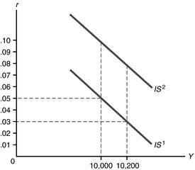
When Y = 10,000,
8000r = 8400 – (0.8 × 10,000) = 400,  so r = 0.05.

When Y = 10,200,
8000r = 8400 – (0.8 × 10,200) = 240,  so r = .03

(c) When G = 2400, desired saving becomes Sd = – 6400 + 4000r + 0.8Y. Sd is now 400 less for any given r and Y.

Setting Sd = Id, we get

– 6400 + 4000r + 0.8Y = 2400 – 4000r

8000r = 8800 – 0.8Y.

Similarly, using the alternative form of the equation gives:

Y = Cd + Id + G
Y = (4000 – 4000r + 0.2Y) + (2400 – 4000r) + 2400
Y = 8800 – 8000r + 0.2Y
So 0.8Y = 8800 – 8000r, or
8000r = 8800 –  0.8Y

At Y = 10,000, this is 8000r = 8800 – (0.8 × 10,000) = 800, so r = 0.10. The market-clearing real interest rate increases from 0.05 to 0.10.

Thus the IS curve shifts up and to the right from IS1 to IS2 in the figure below.

 

2.  (a) Md/P = 3000 + 0.1Y – 10,000i
= 3000 + 0.1Y – 10,000(r + pe)
= 3000 + 0.1Y – 10,000(r + .02)
= 2800 + 0.1Y – 10,000r

Setting M/P = Md/P:

6000/2 = 2800 + 0.1Y – 10,000r
10,000r = – 200 + 0.1Y
r = – 0.02 + (Y/100,000)

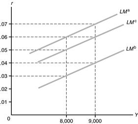
When Y = 8000, r = 0.06.
When Y = 9000, r = 0.07.
(b) M = 6600, so M/P = 3300. Setting money supply equal to money demand:

          3300 = 2800 + 0.1Y – 10,000r
10,000r = –500 + 0.1Y
          r = –0.05 + (Y/100,000)

          When Y = 8000, r = 0.03.
When Y = 9000, r = 0.04.

          The LM curve is shifted down and to the right because the same level of Y gives a lower r at equilibrium.

     (c)  Md/P = 3000 + 0.1Y – 10,000(r + pe)
= 3000 + 0.1Y – 10,000r – (10,000 ´ .03)
= 2700 + 0.1Y – 10,000r.

     Setting money supply equal to money demand:
3000 = 2700 + 0.1Y – 10,000r
10,000r = – 300 + 0.1Y
          r = – 0.03 + (Y/100,000).
When Y = 8000, r = 0.05.
When Y = 9000, r = 0.06.

     The LM curve is shifted down and to the right

          

 

3.  Step 1: Find the IS Curve.  Begin by finding the savings curve:
S = Y – C – G
S = Y – (200 + .8Y - .8T – 500r) – 196
S = Y – 200 - .8Y + .8(20 + .25Y) + 500r – 196
S = .2Y – 396 + 16 + .2Y + 500r
S = .4Y – 380 + 500r
Next set S = I:
.4Y – 380 + 500r = 200 – 500r
.4Y = 580 – 1000r
Y = 1450 – 2500r   (This is the equation for the IS curve.)

 

Step 2: Find the LM curve
Ms/P = Md/P
9890/P = .5Y –250(r + .1)
9890/P + 250r + 25 = .5Y
Y = 19780/P + 500r + 50  (This is the equation for the LM curve)
Step 3:  Solve for r, P, C and I
The economy is at full employment output, which is given as 1000.  Using the IS curve, we can find r:
Y = 1450 – 2500r
1000 = 1450 – 2500r
2500r = 450  so r = 450/2500 = .18
Given Y and r, we can find P on the LM curve:
Y = 19780/P + 500r + 50
1000 = 19780/P + 500(.18) + 50
1000 = 19780/P + 140
860 = 19780/P   
P = 19780/860 = 23
Step 4:  Find C and I
C = 200 + .8[1000 – (20 + .25(1000)] –500(.18)
C = 694
I = 200 – 500(.18) = 110
Analytical problems
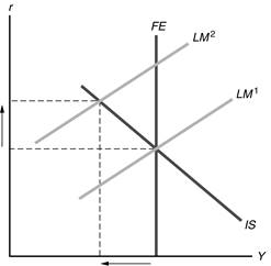
3.  (a) The decrease in expected inflation increases real money demand, which shifts the LM curve left (up). The real interest rate rises and output declines, as illustrated in the following diagram:

(b)  The increase in desired consumption shifts the IS curve up and to the right, as shown below.  The real interest rate and output both rise.

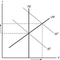
(c)  The increase in government purchases shifts the IS curve up and to the right.  The result is the same as in part (b).
(d)  If Ricardian equivalence holds, the increase in taxes has no effect on either the IS or LM curves, so there is no change in either the real interest rate or output. If Ricardian equivalence doesn’t hold, the increase in taxes reduces consumption spending.  The IS curve shifts down and to the left. as shown in the following diagram. Both the real interest rate and output decline.

(e)  An increase in the expected future marginal productivity of capital will increase investment.  The IS curve shifts right, with the same result as in part (b).

Chapter 11
Review Questions
1.   The efficiency wage is the real wage that maximizes effort or efficiency per dollar of real wages. It assumes that workers will exert more effort, the higher the real wage. The real wage will remain rigid even if there is an excess supply of labor, because firms won’t reduce the wage they pay; doing so would reduce their profits, since workers wouldn’t work as hard.
2.   Full-employment output is the amount of output produced by firms with employment determined by the labor demand curve at the point where the marginal product of labor equals the efficiency wage.
A productivity shock does not lead to a change in the efficiency wage, since it does not affect work effort. But it does affect the marginal product of labor, so employment changes. A beneficial productivity shock, for example, leads to an increase in employment. Both the employment increase and the increase in productivity lead to an increase in full-employment output.
Labor supply changes have no effect on the efficiency wage or employment; they simply affect the amount of unemployment. So they have no impact on full-employment output.
3.   Price stickiness is the tendency of prices to adjust only slowly to changes in the economy. Keynesians believe it is important to allow for price stickiness to explain why monetary policy is not neutral.
4.   Menu costs are the costs of changing prices. Menu costs may lead to price stickiness in monopolistically competitive markets but not in perfectly competitive markets, because a monopolistically competitive firm’s demand is not as sensitive to the price as is a perfectly competitive firm’s demand. Monopolistically competitive firms may meet the demand at a fixed price when demand increases, because price exceeds marginal cost, so that profits still rise, and because the cost of changing prices may exceed the additional profit earned from doing so. A perfect competitor would lose all of its customers if its price were a little above the price charged by its competitors. But a monopolistically competitive firm would lose only some of its customers in this case.
6.   In the Keynesian model in the short run, output and the real interest rate increase due to an increase in government purchases. In the long run, the real interest rate is higher, but output returns to its full-employment level. Since the real interest rate is higher in the long run, investment is lower and consumption is lower.
10. In Keynesian analysis, a supply shock may reduce output in two ways: (1) a reduction in output, because the supply shock reduces the marginal product of labor, shifting the FE line to the left; and (2) a further reduction in output if the supply shock is something like an oil price shock that is large enough to cause many firms to raise prices, shifting the LM curve up and to the left so much that it intersects the IS curve to the left of the FE line. Supply shocks create problems for stabilization policy because: (1) policy can do nothing to affect the location of the FE line; and (2) using expansionary policy risks worsening the already-high rate of inflation.

Numerical Problems

1.   The following table shows the real wage (w), the effort level (E), and the effort per unit of real wages (E/w).

w	E	E/w
8	7	0.875
10	10	1.00
12	15	1.25
14	17	1.21
16	19	1.19
18	20	1.11

      The firm will pay a wage of 12, since that wage provides the maximum effort per unit of the real wage (E/w = 1.25). The firm will employ 88 workers, since that is the number of workers for which
w = MPN. That’s because MPN = E(100 – N)/15.  When w = 12, E = 15, so w = MPN  implies 12 = 15(100 – N)/15.  N therefore = 88.  As long as the supply of labor exceeds the demand for labor, labor supply has no effect on the firm’s decision.

 

3.   The IS curve is Y = Cd + Id + G = [600 + 0.8(Y – 1000) – 500r] +[400 – 500r] + 1000, so 0.2Y = 1200 – 1000r. This is plotted in Figure 11.12.

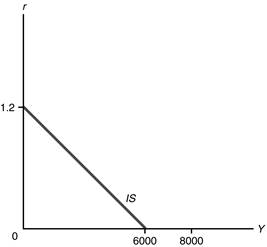
Figure 11.12
Since pe= 0, the nominal interest rate (i) equals the real interest rate (r).
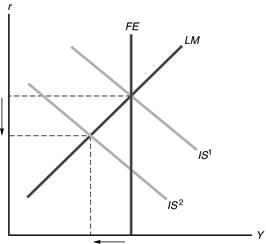
(a) Can the economy reach full employment? Since full-employment output is Y = 8000, for the economy to be on the IS curve, 0.2Y = 1200 – 1000r, so (0.2 ´ 8000) = 1200 – 1000r, or 1000r = –400, so r = i = –.4. But since the nominal interest rate can’t be negative, this isn’t possible. Thus, the requirement that i be non-negative means that there’s no way to satisfy the goods markets equilibrium condition at full employment. Assuming that the result is that i = 0 and that output is determined along the IS curve, 0.2Y = 1200 – (1000 ´ 0), so Y = 6000. Note that this is the best result possible, no matter what the money supply is, so monetary policy can’t restore full employment.
(b) To restore full employment while the nominal interest rate is zero clearly requires a shift in the IS curve. If we return to the original derivation and put G in the equation instead of using the original value of G = 1000, we get:
Y = Cd + Id + G = [600 + 0.8(Y – 1000) – 500r] +[400 – 500r] + G, so 0.2Y = 200 + G – 1000r. To get Y = 8000 and r = 0, we have 0.2 ´ 8000 = 200 + G – (1000 ´ 0), so G = 1400. Then the IS curve is 0.2Y = 1600 – 1000r. This is plotted in Figure 11.13 as IS2, while the original IS curve is IS1.

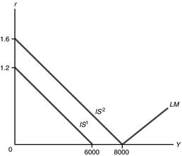
Figure 11.13
Thus, raising G to 1400 can generate full employment, if the money supply is chosen so that the LM curve intersects the IS curve at the right point. Note that taxes are 1000, so the government must run a large budget deficit.
What must the money supply be? Since P = 2, we need money supply (M/P) = money demand (L), so M/2 = 0.5Y – 200i = (0.5 ´ 8000) – (200 ´ 0) = 4000, so M = 8000.
This situation is quite similar to the situation in Japan in the 1990s and suggests that to get out of the liquidity trap, Japan will need to use expansionary monetary policy, along with expansionary fiscal policy.

Analytical Problems

1.   a.  The tax incentive for investment shifts the IS curve to the right. The short-run effect is to increase output, employment and the real interest rate; the price level is unaffected.  In the long-run, the price level will rise, and that will shift the LM curve left.  Relative to the starting point, output and employment will be the same, but the price level and interest rate will be higher.

      b.  The tax incentive for saving reduces consumption, so the IS curve shifts left. The short-run effect is to reduce output, employment and the real interest rate; the price level is unaffected.  In the long-run, the price level will fall, and that will shift the LM curve right.  Relative to the starting point, output and employment will be the same, but the price level and interest rate will be lower.

      c.  Investor pessimism about future profits will reduce investment and shift the IS curve left. The short-run effect is to reduce output, employment and the real interest rate; the price level is unaffected.  In the long-run, the price level will fall, and that will shift the LM curve right.  Relative to the starting point, output and employment will be the same, but the price level and interest rate will be lower.

      d.  Higher consumer confidence will increase consumption and shift IS to the right. The short-run effect is to increase output, employment and the real interest rate; the price level is unaffected.  In the long-run, the price level will rise, and that will shift the LM curve left.  Relative to the starting point, output and employment will be the same, but the price level and interest rate will be higher.

 

Chapter 13
Review questions
1.  The nominal exchange rate is the rate at which two currencies can be exchanged for each other in the market. The real exchange rate is the price of domestic goods relative to foreign goods. Changes in the two exchange rates are related as follows:
% change in enom= % change in e + Pfor - PUS
2.   The two major types of exchange-rate systems are fixed exchange rates and flexible exchange rates. In a fixed-exchange-rate system, exchange rates are set at officially determined levels. In a flexible-exchange-rate system, exchange rates are determined by conditions of demand and supply in the foreign exchange market. Currently, the major currencies of the world are on a flexible-exchange-rate system (more or less).

3.  Purchasing power parity, PPP, is the idea that similar foreign and domestic goods, or baskets of goods, should have the same price when priced in terms of the same currency. Purchasing power parity does seem to explain exchange rates in the long run, but over shorter periods it doesn’t work well because countries produce very different sets of goods, because some goods aren’t traded internationally, and because there are transportation costs and legal barriers.

4.  The J curve shows the response of net exports to a real depreciation. At first the real depreciation reduces net exports, as the decline in the real exchange rate means that a country pays more for its imports and receives less for its exports. But as time passes, the higher price of imports reduces the demand for imports, while the lower price of the country’s exports increases their demand abroad. So eventually net exports begin to increase.

5.  An increase in domestic income leads people to buy more goods, including imported goods, so net exports decline. An increase in foreign income leads foreigners to buy more goods, including goods exported from the domestic country, so net exports increase. An increase in the domestic real interest rate makes domestic assets more attractive and foreign assets less attractive to both domestic and foreign investors. This causes a reduction in the supply of the domestic currency on the foreign exchange market and an increase in demand for the domestic currency on the foreign exchange market. The result is an appreciation of the domestic currency, which leads to a decline in net exports.
6.   Foreigners demand dollars in the foreign exchange market to be able to buy U.S. goods and services (U.S. exports) and U.S. real and financial assets (U.S. capital inflows). Americans supply dollars to the foreign exchange market to be able to buy foreign goods and services (U.S. imports) and real and financial assets in foreign countries (U.S. capital outflows). The demand for dollars increases if the demand for U.S. goods increases, the domestic real interest rate increases, foreign income increases, or the foreign real interest rate decreases. The supply of dollars increases if the demand for foreign goods increases, the domestic real interest rate decreases, domestic income increases, or the foreign real interest rate increases.

7.   The IS-LM model for the open economy differs from the closed-economy IS-LM model in that international influences may shift the IS curve. Factors that raise a country’s net exports, given domestic output and the domestic real interest rate, shift the IS curve upward, while factors that reduce a country’s net exports shift the IS curve downward. A recession could be transmitted from one country to another because a recession in one country reduces the net exports of other countries, shifting their IS curves down. In the Keynesian model in the short run, this would lead to a reduction in output in the other countries.

8.  Expansionary fiscal policy increases output and the real interest rate in the short run, both of which lead to a reduction of net exports. Expansionary monetary policy increases output in the short run, which tends to reduce net exports, but reduces the real interest rate, which tends to increase net exports (by reducing the exchange rate). The overall effect is potentially ambiguous, but the effects of changes in the real exchange rate on net exports may be weak in the short run, so it is likely that net exports will decline.

Numerical problems

4.  a.  General equilibrium output is given as 1,000.
The IS curve is given by the equation
S – I = NX
S = Y – C – G = Y – [200 + .6(Y – T) – 200r] – 152
S = Y – 200 - .6Y + .6(20 + .2Y) + 200r – 152
S = .52Y – 340 + 200r

          S – I = .52Y – 340 + 200r – 300 + 300r
S – I = .52Y – 640 + 500r

          NX = 150 - .08Y – 500r (given)

          S – I = NX
.52Y – 640 + 500r = 150 - .08Y – 500r
.6Y = 790 – 1000r
Y = 1316.67 – 1666.67r  (IS curve)

          Since Y is given at 1000, one can solve for r with only the IS curve:

          1000 = 1316.67 – 1666.67r

          r = .19

          The LM curve is given by the equation

         Ms/P = Md/P

         924/P = .5Y – 200r

         Given Y and r, one can solve for P using the LM curve:

         924/P = .5(1000) – 200(.19)

         P = 2

          Plugging Y = 1000 and r = .19 into the C, I and NX:

          C = 630      I = 243        NX = -25

     b.  G = 214 changes S to

S = .52Y – 402 + 200r

          repeating the derivation in part (a), the new saving functions gives:

          S – I = NX

          .52Y – 702 + 500r = 150 - .08Y – 500r

          .6Y = 852 – 1000r

          Y = 1420 – 1666.67r  (new IS curve)

          The LM curve is the same.  In the short run P = 2 so

          924/2 = .5Y – 200r

          Y = 924 + 400r (LM curve with P = 2)

     The IS and LM curves together give us two equations and two      unknowns.  Solve them together to find short run equilibrium Y and r:

     IS:  Y + 1666.67r = 1420
LM: Y – 400r = 924

     Subtract LM from IS

     2066.67r = 496
r = .24

     Plugging r into either equation gives us Y = 1020

     Plugging r and Y into the appropriate equations gives:

     C = 629.6   I = 228        NX = - 51.6

In the long run, Y returns to 1000, so

         The IS curve is Y = 1420 – 1666.67r or

         1000 = 1420 – 1666.67r so

         r = .25

         Plugging  Y and r into the LM curve gives us

         924/P = .5Y – 200r or

         924/P = .5(1000) – 200(.25)

         so P = 2.055

         The long run values for C, I and NX are:

         C = 618       I = 225        NX = -55